The Argument I Never Tested
This is a companion to One Crisis Deep.
I.
Since May, the Regime Radar page has carried a short section explaining why it sorts markets with two plain rules instead of a hidden Markov model, the tool most papers on regime detection reach for. It gave three reasons, which read like this:
- “The labels move. Refit with one more day of data and the model can relabel months of history.”
- “The states have no fixed meaning. State 0 in one fit can be state 1 in the next.”
- “The probabilities look more precise than they are.”
They sound right, and they read like the kind of thing that has been checked. A few days ago I rewrote the page into English, tidied the prose and kept all three. I didn’t check any of them.
That’s awkward, because the same week I wrote a whole post about pre-registering a test so I couldn’t fool myself. Meanwhile my own site had been making three empirical claims for four months with no evidence behind them. The claims sat in the part of the page nobody questions, the part that explains why I didn’t do the other thing.
So I tested them.
II.
A hidden Markov model assumes the market is always in one of a few unobserved states, each with its own typical daily return and volatility, and that it jumps between them with fixed probabilities. You never see the state. You fit the model to the returns, and it tells you, for every day, how likely each state was.
With two states on IHSG since 2005, the model finds what you’d expect: a calm state with daily swings of about 0.8% that lasts 55 trading days on average, and a turbulent one with swings of about 2.3% that lasts 14. It puts 18% of days in the turbulent state, about a third of them in 2008 and 2009 alone.
To test the page fairly, the model gets the strongest setup I could give it rather than a strawman:
- Each fit is the best of five random starting points.
- After every fit the states are sorted by volatility, so “turbulent” always means the most volatile one.
- It is refit at every month end from 2010, using only data up to that day.
- Each day gets a real-time label from a forward filter, run with the parameters from the most recent refit. The filter only uses data up to that day, which is how you would run the model live.
Then the question for each claim is simple: when the model gets more data, what happens to what it said about the past?
III.
Start with the first claim and the two-state model, because that’s the version most people draw.
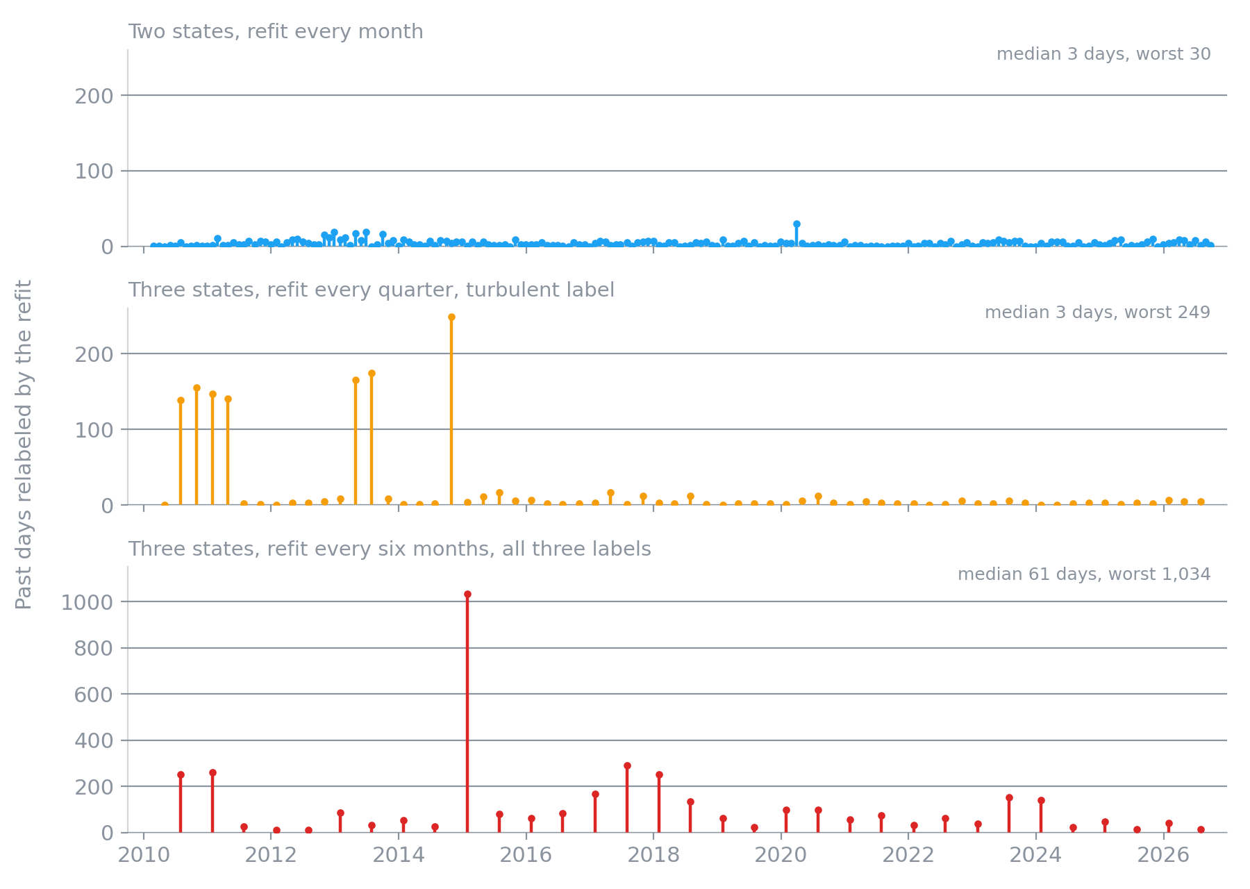
How many past days each refit relabeled. Top: two states, monthly. Middle: three states, quarterly, turbulent label only. Bottom: three states, every six months, all three labels. Note the different scale.
The labels do move. Of 200 monthly refits, 178 changed at least one past day, and the changes reach a long way back: the earliest day a refit changed was typically about ten years in the past. But the amount is tiny. The median refit relabeled 3 days out of several thousand. The worst relabeled 30, under 1% of the history at the time, and it came at the end of March 2020, right after the COVID crash. The probabilities behind the labels moved by a median of 0.14 percentage points. Refitting after every single day for the last year made it smaller still: 138 of the 250 daily refits changed nothing at all, and the worst changed 14 days.
“Refit with one more day of data and the model can relabel months of history” is false for this model. It relabels a few borderline days, the ones sitting right at 50% between calm and turbulent, and leaves the rest alone.
One more thing I expected to matter, and it didn’t: fitting from a single random start instead of the best of five gave identical results, to the last digit. With two states the model lands on the same answer whatever you feed it at the start.
IV.
Then I asked for three states, and the first claim came back.
A three-state model on IHSG finds a calm state, a normal one and a turbulent one. Even looking only at the turbulent label, refit every quarter, most refits change a handful of days as before, but a few rewrite a lot: 10% of refits relabeled at least 4.7% of history, and the worst relabeled 249 days, close to a year. Look at all three labels, refit every six months, and it gets much worse. The median refit relabeled 61 days, and one refit relabeled 1,034 days, 46% of everything the model had seen.
The reason is visible in the fitted states. The calm and normal states have daily volatilities of 0.6% and 1.1%, close enough that many days fit either one about equally well. When new data nudges the parameters, whole stretches of history flip from calm to normal and back. The turbulent state, at 2.7%, is different enough to stay put, which is why the two-state model is stable: it only has to separate the obvious.
The timing is worth noticing too. In the middle panel of the figure, the big rewrites of the turbulent label all came between 2010 and 2014, when the model had five to nine years of data, and after that it settled. For that label, instability was worst when the model was newest, which is usually when people start trusting a new model. The split between calm and normal never settled at all. Its worst refit, the one that relabeled 46% of history, came at the start of 2015, and refits in 2017, 2018, 2023 and 2024 still rewrote between 134 and 290 days each.
So the page’s first claim is true, just not for the model I had in mind. It holds for the richer model people like to draw, the one with bull, bear and sideways regimes, and it barely holds for the simple one.
V.
The second claim, that state 0 in one fit can be state 1 in the next, is true. Across the 199 pairs of consecutive monthly refits, the raw index of the turbulent state swapped 95 times, about as often as a coin flip. The model has no idea which of its states you’d like to call “turbulent”.
It’s also the least interesting problem on the list, because one line of code fixes it: after each fit, sort the states by volatility. That’s what every result in this post already does. The claim belongs in a footnote, not in a list of reasons.
VI.
The third claim was that the probabilities look more precise than they are, because the model assumes returns are Gaussian and IHSG’s returns are not. The second half of that is true. Daily IHSG returns since 2005 have an excess kurtosis of 8.6, far fatter tails than a normal distribution. But the model doesn’t assume returns are Gaussian overall. It assumes they’re Gaussian within each state, and the mixture of a calm and a turbulent Gaussian is itself fat-tailed. Measured within the states, the excess kurtosis drops to 0.6 with two states and 2.0 with three. Most of the fat tails turn out to be regime switching, which is the thing the model is built to capture.
The overconfidence part is harder to test, because nobody knows the true state on any given day. The best I can do is ask whether the model’s real-time confidence held up once it saw more data. Over 4,038 days from 2010, the real-time label agreed with the final full-history label 95% of the time. On the 181 days the live model was at least 90% sure of turbulence, the final model agreed every single time. When it was at least 90% sure of calm, the final model agreed 99% of the time. On the days it was unsure, hindsight disagreed about a quarter of the time, which is what “unsure” should mean.
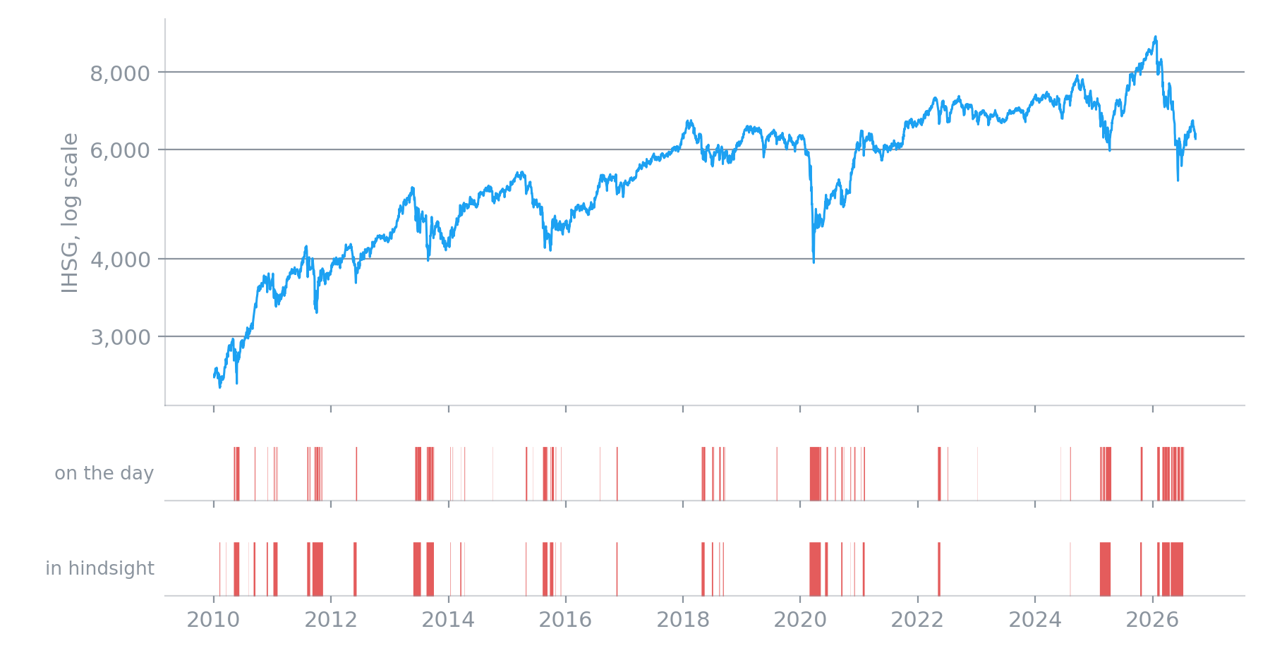
Turbulent days according to the two-state model on the day itself, and according to the model fitted on all data up to September 2026.
This is a check of the model against itself, not against the truth, so it can’t prove the probabilities are calibrated. It does show that they aren’t fragile, and I had claimed they were. The one real gap is small: the live model saw turbulence on 10.4% of days, while hindsight sees 12.2%. The textbook chart, drawn with all the data, shows a little more turbulence than anyone could have seen at the time.
The real-time labels are also informative. After a day the live model called turbulent, the next month’s volatility had a median of 23.2%; after a calm day, 12.7%. Regime Radar’s own volatility label separates next month into 11.5% after low and 17.0% after high over the same years. That isn’t a like-for-like comparison, since the HMM’s turbulent state covers about a tenth of days and Regime Radar’s high band about a third, but it’s enough to say the model is not decoration.
VII.
Tally it up. For the two-state model the page claimed three things: the first is mostly false, the second is true and trivial, and the third isn’t supported. For the three-state model the first claim holds, strongly.
What’s left of the case for rules is shorter than the page said, and I think more honest:
- A rule’s label never changes after the fact. The HMM’s changes are small for two states, but they’re never zero.
- Anyone can check a rule with a spreadsheet. Checking an HMM label means refitting the model.
- A rule can give three regimes without the instability that three HMM states bring. The three-state model is where the HMM case really breaks down.
And one concession: a two-state HMM, run in real time and refit monthly, is a reasonable alternative for telling calm from turbulent. The page’s roadmap had listed “an experimental HMM panel” since May, half as a gesture, so I built it. It sits under the chart as a separate strip, showing only what the model said on each day at the time, and every monthly model it uses is published next to the data.
Building it turned up one more result. For USD/IDR, the same model’s turbulent state lasts about five trading days on average, which makes it a detector of single jumps rather than a regime, so the strip is left out for that series. The panel only appears where the model finds spells of at least ten days, which today means IHSG and the S&P 500.
I’ve rewritten that section of the page to say all this, with the numbers.
VIII.
The three claims were easy to believe because they were in the right place. Nobody audits the paragraph that explains why a road wasn’t taken; the reader has no reason to walk down it, and neither did I. That makes it the natural home for the claims that have never been tested.
Testing all three took under a quarter of an hour of computer time. The paragraph had been on the page for four months.
Code: hmm_refit.py in the site’s repository. It reads the same cleaned IHSG data the dashboard publishes, so the results can be rerun without any download. The docstring lists the three commands behind the numbers above.